Optimizers

Optimization plays a crucial role in science and research, typically involving an objective function that we aim to minimize or maximize. Often, these functions lack an analytic form. For example, optimizing the strength and position of focusing magnets on an accelerator beamline to achieve the smallest electron beam spot size at an interaction point in the presence of space charge requires running (slow) simulations to sample function values.

Ideally, we want to optimize our objective with minimal function evaluations while avoiding local extrema. These are the same challenges encountered when optimizing parameters during the training of a machine learning model. The objective function might be convex (as in linear models) or have multiple extrema (as in neural networks). It is important to have an understanding of different optimization methods and how they compare.

Gradient Descent

The simplest optimization method is gradient descent. If you recall from Calculus, the gradient of a function is a vector composed of partial derivatives in each direction. This gradient vector points toward the direction of maximum increase in the objective function. A common analogy is hiking on a mountain where the gradient points uphill at your current location (but doesn’t necessarily point directly to the summit). One strategy to find the summit is to move in the direction of the gradient a little ways, then compute a new gradient and move in that direction. The distance we move is determined by the learning rate parameter, \( \alpha\). If we want to minimize a function, we apply the same procedure, but more in the opposite direction of the gradient.

Let's define a cost function, \( J(\theta) = \frac{1}{2m} \sum_{i=1}^{m} \left( h_{\theta}(x^{(i)})-y^{(i)}\right) \), as the mean squared error over a training set with our model \( h_{\theta}(x) \) parametrized by a vector \( \theta \). Instead of computing the gradient using the entire dataset at each iteration, we can use a single data point (stochastic gradient descent) or a subset of the data (mini-batch gradient descent) to speed up computation. This approach also introduces noise, which can help avoid local minima. At each iteration, the parameters are updated according to the rule

\( \theta_j = \theta_j - \alpha v_j \)

Momentum

One limitation of gradient descent is that it uses only information from the current position. If our function has a gentle slope toward the minimum, gradient descent takes small steps, resulting in slow convergence. Ideally, we want the optimizer to behave like a rolling ball, gaining speed and taking larger steps as the gradient points in the same direction. We can incorporate this concept of momentum into the update rule by accumulating knowledge of the previous velocities, which improves optimization when dealing with gentle slopes or noisy gradients.

\( v_j = \beta v_j + (1 - \beta) \frac{\partial J}{\partial \theta_j} \)

\( \theta_j = \theta_j - \alpha v_j \)

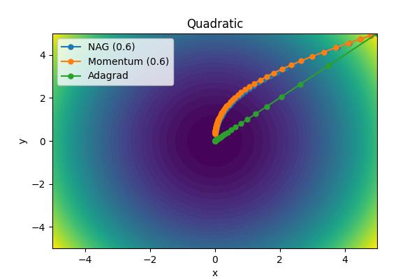
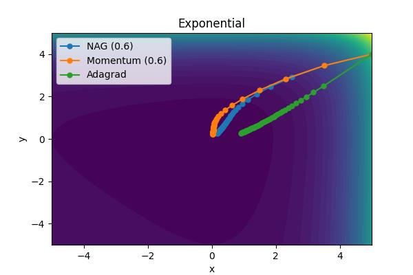
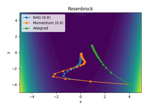
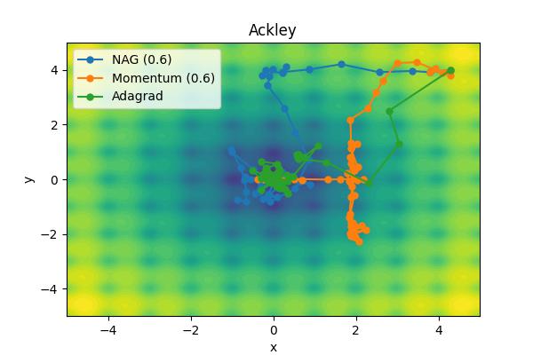
The momentum parameter, \( \beta \), controls how previous velocities and current gradient contribute. Note that for \(\beta=0\), we recover simple gradient descent. On the other hand, in the limit \(\beta=1\) we throw away gradient information completely. The following images show the performance for a few different analytic cost functions where the minimum is at 0,0. In this case, we are using \(\theta = [x, y]\).

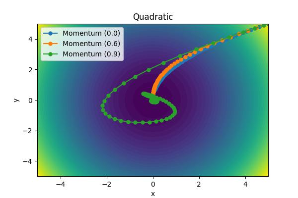
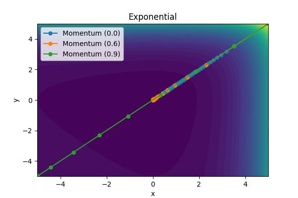
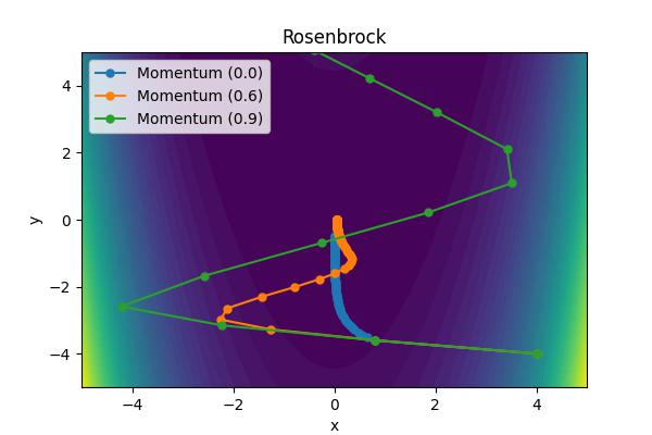
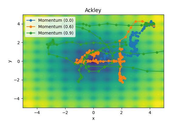
Aside from the Ackley cost function with many local extrema, it is clear the gradient descent algorithm works, but takes an unnecessarily long time to convert. Increase the moment parameters leads to significant improvements. When the momentum parameter is too large, the optimizer can (wildly) overshoot the minimum. Of course I have tweaked scalings to demonstrate the different behaviors. It is not always obvious what the momentum parameter should be set to.

Nesterov Accelerated Gradient (NAG)

The NAG optimizer is an improvement over the standard momentum optimizer. The basic idea is to use a "look-ahead" mechanism, \( \theta_j' = \theta_j + \beta v_j \), to compute the gradient at the future position instead of the current position. This can accelerate the convergence when the optimization surface is curved. The velocity and position are then updated according to

\( v_j = \beta v_j + \alpha \frac{\partial J}{\partial \theta_j'} \)

\( \theta_j = \theta_j + v_j \)

Adaptive Gradient Algorithm (Adagrad)

Adagrad is an optimization algorithm that adapts the learning rate for each parameter individually. This allows the algorithm to perform well on surfaces with different slopes in each direction. The scaling for each learning rate is determined by the accumulated squared gradients, \( G_j = G_j + (\frac{\partial J}{\partial \theta_j})^2 \) with the update rule given by

\( \theta_j = \theta_j + \frac{\alpha}{\sqrt{G_j}+\epsilon} \frac{\partial J}{\partial \theta_j} \)

The \( \epsilon \) is a small value (1e-8) to avoid division by zero. Another optimizer called Root Mean Square Propagation (RMSP) is very similar to Adagrad, but tries to improve by using an exponential moving average (see next section) rather that a cumulative sum of squared gradients.

By using the advanced gradient, the NAG algorithm takes a straighter path to the minimum than the Momentum algorithm. On the other hand, by adjusting the step in each dimension Adagrad can take a nearly straight path to the minimum. The comparison is not exact as I tweaked the nominal \( \alpha \) in Adagrad, but these images clearly show the effects of different optimization strategies.

Adam

Why not combine the concepts of moment and adaptive learning rates in one algorithm? That is the idea behind the Adam optimizer which is specifically popular for training neural networks. We initialize the two variables \(m_j\) and \(v_j\) (initially zero) to track the exponential moving average of the first and second derivative powers.

\( m_j = \beta_1 m_j + (1-\beta_1) \frac{\partial J}{\partial \theta_j} \)

\( v_j = \beta_2 v_j + (1-\beta_2) \left(\frac{\partial J}{\partial \theta_j}\right)^2 \)

Iterating a few times, \(m_j = \beta_1^2(1-\beta_1)\frac{\partial J}{\partial \theta_j}\Big|_{\theta_{j0}} + \beta_1(1-\beta_1)\frac{\partial J}{\partial \theta_j}\Big|_{\theta_{j1}} + (1-\beta_1)\frac{\partial J}{\partial \theta_j}\Big|_{\theta_{j2}} \), the exponential decay is clear. Because these variables are intialized to zero, they have a tendency to be biased towards 0 if \( \beta\approx 1\). For this reason (and to control oscillations near the global minimum), the parameters are scaled before updating the weights.

\( \hat m_j = \frac{m_j}{1-\beta_1} \)

\( \hat v_j = \frac{v_j}{1-\beta_2} \)

\( \theta_j = \theta_j - \hat m_j \left( \frac{\alpha}{\sqrt{\hat v_j} + \epsilon}\right) \)

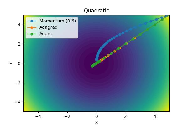
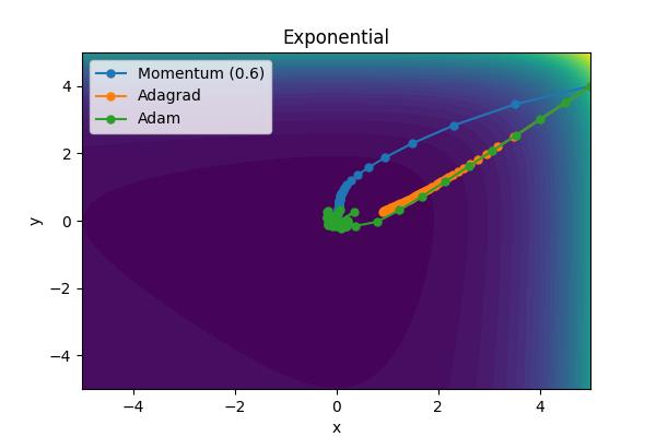
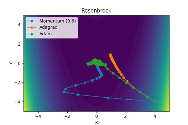
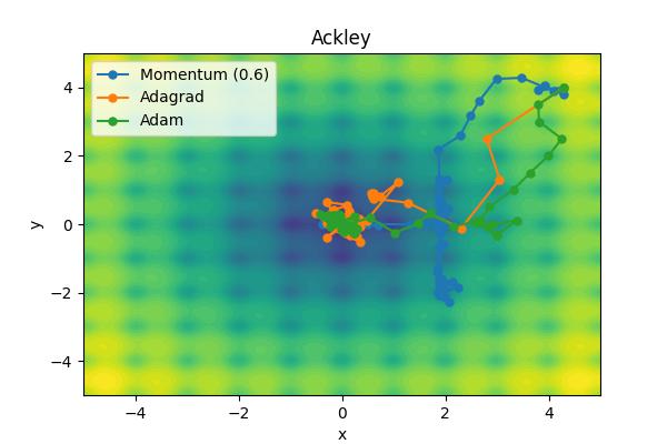
The performance of Adam is outstanding. What jumps out to me the most is that it is able to head directly toward the global minimum with relatively equal sized steps unlike Adagrad or the Momentum solver.